Thesis Master's Thesis (IDSIA / USI) 2017

What Neural Networks Reveal While They Learn

Dhananjay Tomar

Master's Thesis (IDSIA / USI) · 2017

Published 30 June 2017

📄 Thesis 💻 Code

Adding Gaussian noise to CIFAR-10 images causes Highway Networks to open their transform gates more, showing that the network learns to allocate more computation to more difficult samples. The blue curve is the clean input; green, red, and yellow add progressively more Gaussian noise.

Summary

A 2017 study of individual-example and mini-batch dynamics during neural-network training: how quickly examples are learned, how their losses move across epochs, how Highway Networks allocate gated computation, and why apparently sensible curricula can still lose to random shuffling.

A quick note from the author: I wrote this Master's thesis in 2017 and never turned it into a paper. That still feels like a missed opportunity, because several questions I was chasing—tracking individual examples across epochs, using training trajectories to diagnose difficulty, and deciding which examples matter at a particular point in training—became major research themes soon afterward. The later papers used different definitions, broader experiments, and much stronger validation; I am not claiming they are the same work. But the conceptual overlap is real, especially around example forgetting, and it is hard not to wonder what another few months of experiments might have produced.

The original goal was ambitious. I wanted to design a curriculum learning strategy for an NLP task, but as the project evolved, we pivoted to computer vision and CIFAR-10. My supervisor, Klaus Greff at IDSIA, had a clear philosophical vision: we needed an automated curriculum, but we also needed to know why it worked.

We could, for example, have tried to develop a Reinforcement Learning agent to arbitrarily pull examples for the network-which some labs did later-but that creates a black box. If we instead managed to dynamically sort the dataset into "difficult" and "easy" bins based on well-defined mathematical criteria, we would actually understand the fundamental learning process.

Idea 1: The Loss-Drop Cycle (Usefulness vs. Difficulty)

Where to look in the thesis (printed page numbers)

• §4.2.2 and Figs. 4.12-4.15, pp. 40-44: cross-epoch loss changes and the failed greedy curriculum.

My very first idea was simple: high loss equals high difficulty. But difficulty is not the same thing as usefulness. To ask which examples were actually helping at a particular moment, I tracked each example's loss-drop: how much its loss changed from one epoch to the next.

I discovered a fascinating cycle. Consecutive epochs were usually negatively correlated. Examples whose loss had risen tended to receive a massive decrease in the following epoch; examples that had just received a large decrease tended to flatten out.

Figure 4.14: The examples with the largest positive loss-drop in one epoch mostly came from the negative-loss-drop region in the preceding epoch, then moved close to zero.

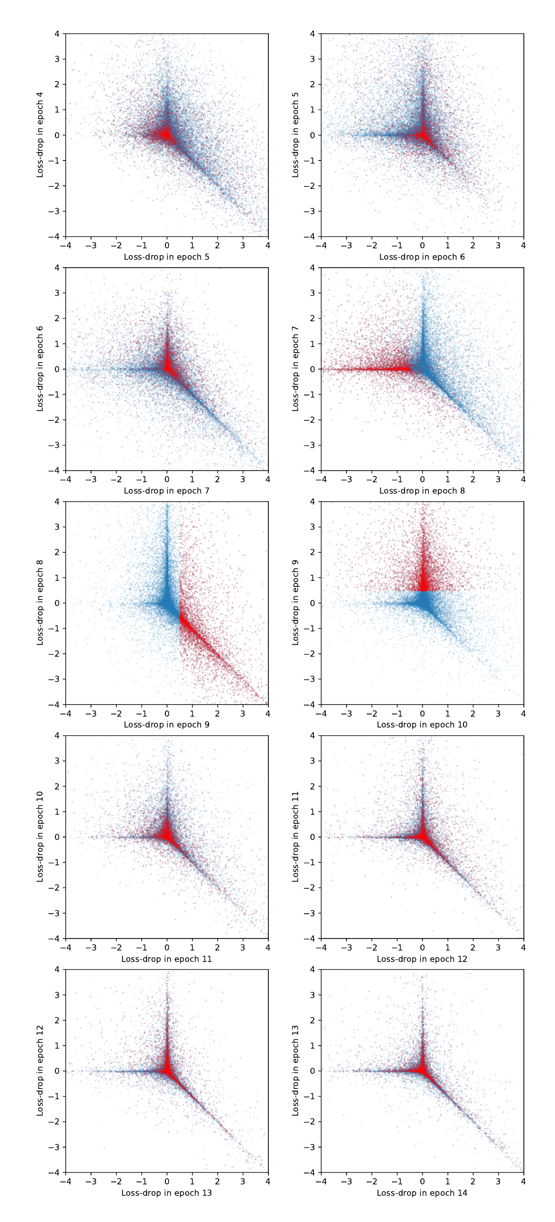
Because we couldn't find any group of examples that stayed difficult, I initially moved on to other ideas. It was only much later, while actually writing the thesis, that I realized we could still exploit this knowledge to design a curriculum. I ran a greedy experiment: select the examples whose loss had just increased, because they were likely to improve most next.

The experiment failed. Training only on that set made other examples worse; two competing groups effectively traded loss back and forth. Selecting 10,000, 20,000, or 30,000 examples prevented convergence; selecting 40,000 converged but still underperformed training on all 50,000. Stratified sampling repaired the class imbalance (easy samples came from a few classes), but only recovered the random baseline rather than beating it.[1] An example can be useful even when its own loss is not about to fall, because its gradient may protect or improve other examples.

Idea 2: Resource-based difficulty (Highway Networks)

Where to look in the thesis (printed page numbers)

• §4.1.1, pp. 24-32: transform-gate activity as a resource-based notion of difficulty.

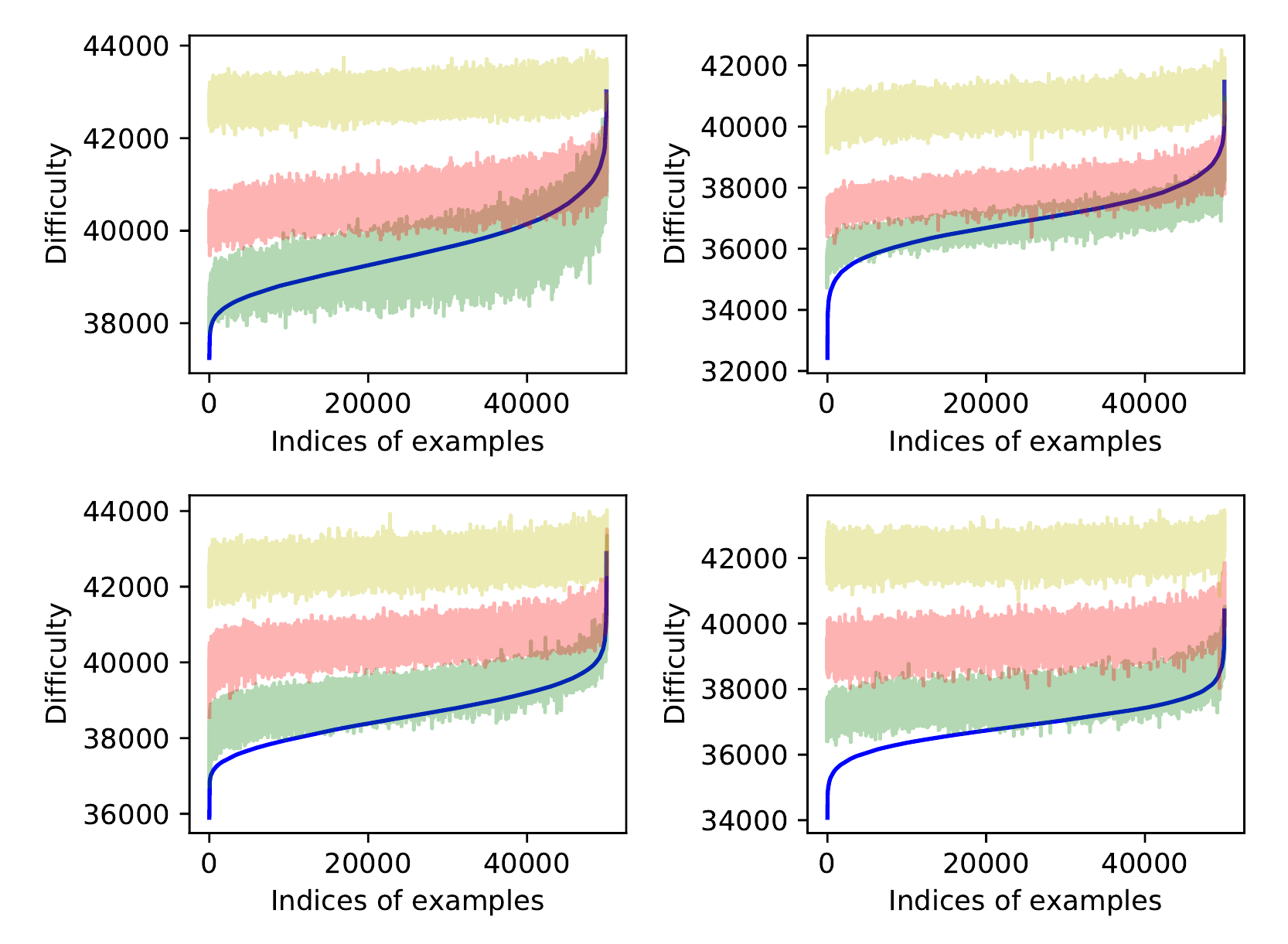
Next, I defined difficulty by how much computation an example activates. Highway Networks contain transform gates. The original papers on Highway Networks had already observed that inherently difficult datasets (like CIFAR) utilize these gates differently than simple datasets (like MNIST). I wanted to take this a step further: could we use these gates to score the difficulty of individual examples within the same dataset?

I treated the sum of these gate outputs as a rough measure of the computation allocated to an example. To test whether that score meant anything, I added increasing amounts of Gaussian noise to CIFAR-10 images.

Figure 4.1: The blue curve is the clean input; green, red, and yellow add progressively more Gaussian noise. Across four runs, more difficult inputs activated more gated computation.

A control network that had never been trained on noise did not show the same behaviour. The effect was therefore not merely a mechanical response to larger or stranger pixel values; the network had learned to route more gated computation toward the kind of difficulty it had encountered during training. Different Highway Network runs also broadly agreed on which examples demanded more of that computation.

The experiment that became a pruning project

There was a loose end. The gates changed with difficulty, but their absolute values remained fairly high and the separation between easier and harder examples was not dramatic. My working theory was simple: the network had no reason to keep a gate closed. If using another transform was free, why not keep using it?

I added an explicit incentive to minimise transform-gate activity. The gate values collapsed—from roughly the 0.45-0.70 range in the ordinary model to around 0.02-0.12 in the incentivised model. Once a transform gate stayed near zero, both the transform branch and its gate could be removed. I pursued this idea later in a high-performance-computing course project at USI, and it became Pruning Highway Networks for Reducing Memory Usage, which I presented as a student poster at PASC17. The pruned model shrank from 34 MB to 5.2 MB—about 85%—for a 1.7 percentage-point accuracy drop.

Idea 3: Time-to-learn and catastrophic forgetting

Where to look in the thesis (printed page numbers)

• §4.1.2, pp. 32-36: time-to-learn and agreement across Highway and All-Conv networks.

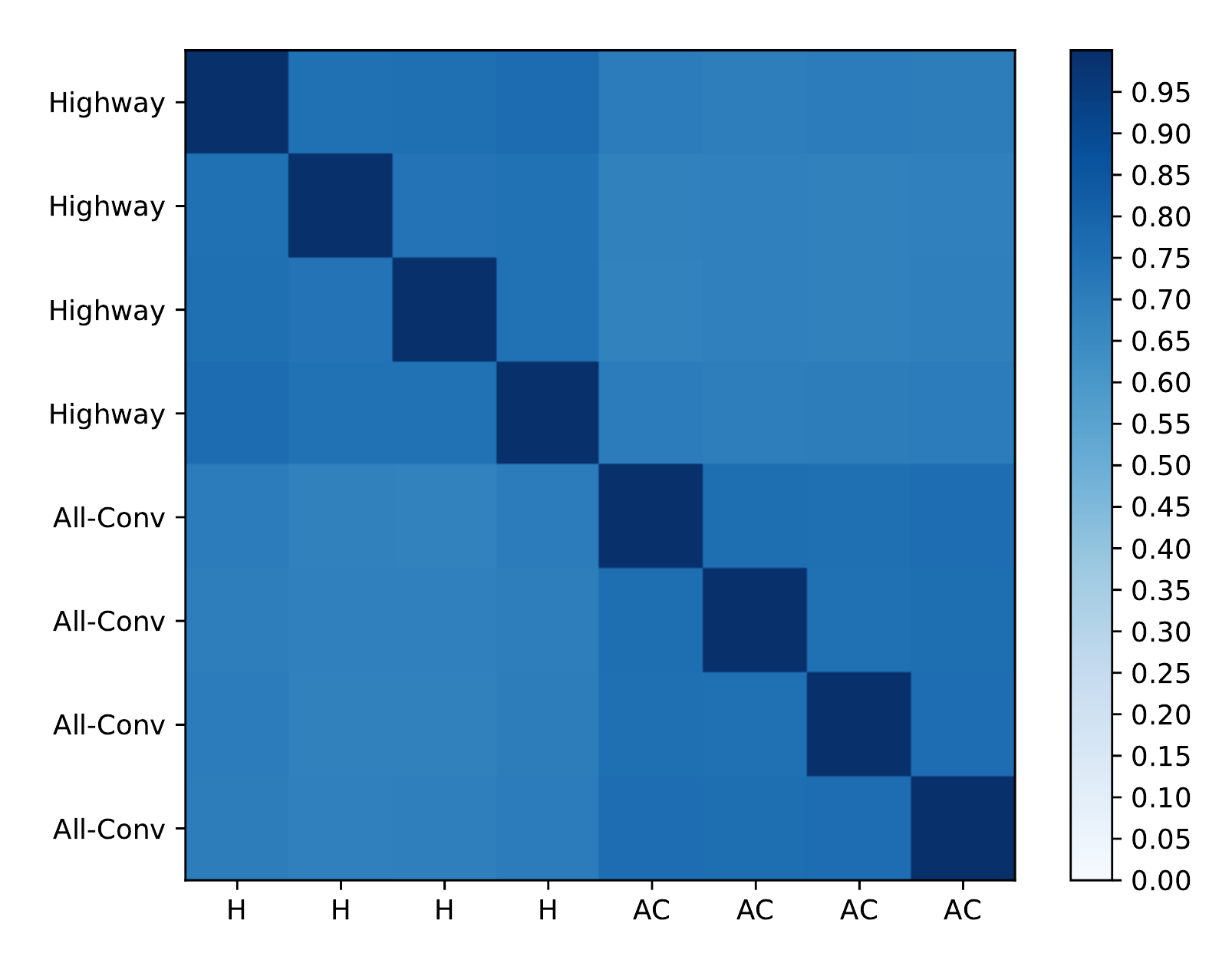
My third definition of difficulty was independent of Highway Networks. For each example, I measured the first epoch at which its loss crossed a confidence threshold. This “time-to-learn” score was correlated not only across random initialisations, but also across two different architectures: Highway Networks and an All-Convolutional network.

Figure 4.7: Examples learned early or late with some consistency across runs and architectures.

I attempted to build a curriculum based on this metric, experimenting with several strategies like starting with the fastest-learning examples. However, some classes became severely under-represented because the network naturally learned certain objects faster than others, leading to catastrophic forgetting. I fixed this by applying stratified sampling, which repaired the class imbalance, but ultimately it only recovered the random baseline rather than beating it.

The ecology of mini-batches

Where to look in the thesis (printed page numbers)

• §4.3 and Figs. 4.16-4.18, pp. 41-50: the “ecology” of how mini-batches affect one another.

I then measured those interactions directly. Starting from a fixed training state, I trained on one mini-batch and recorded the loss change it caused on every other mini-batch. Each source batch was represented by a high-dimensional vector of positive and negative effects. If batches had stable roles, vectors belonging to the same batch should have stayed near one another as training progressed.

Figure 4.17: the batch-effect vectors clustered primarily by epoch—the current state of the model— rather than by a persistent identity of the batch.

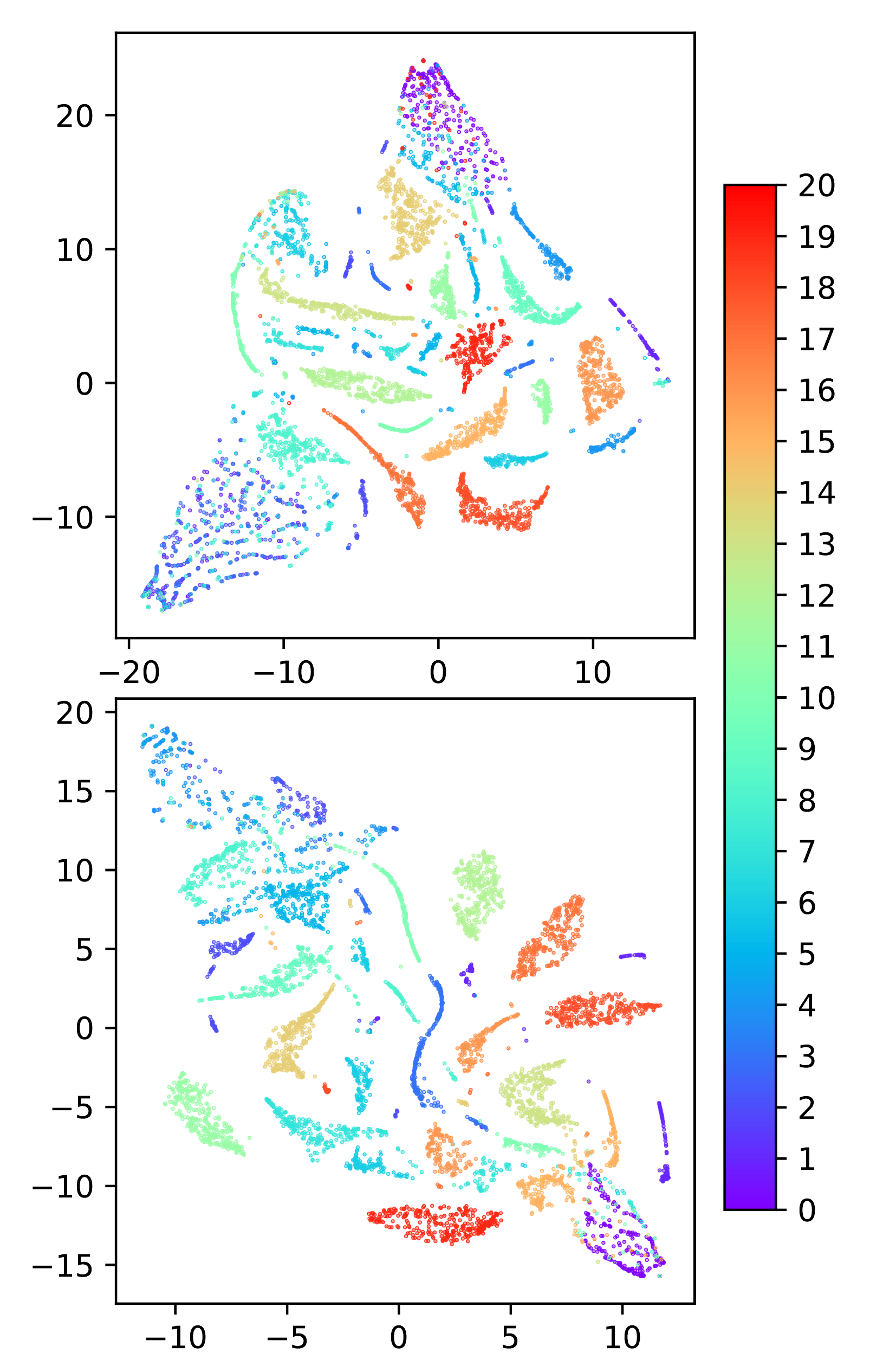
The strongest structure was temporal. Vectors clustered by epoch, and after removing the epoch-level mean and scale, the same batch did not remain in a stable cluster. In this setup, what a batch did to the rest of the dataset depended more on the current parameters than on a permanent property of that batch.[1]

Difficulty was not one axis

The resource-based and time-based scores both looked sensible, and each was reasonably stable on its own, but they did not select the same examples.

Figure 5.1: Two plausible definitions of “hard” agreed only weakly.

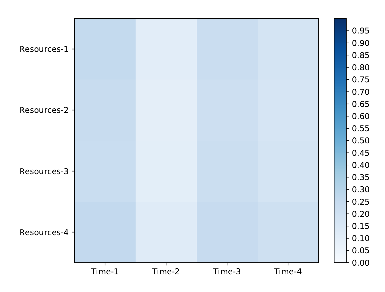
In the language of the thesis, they behaved like different—and approximately orthogonal—dimensions of difficulty. This may help explain why exploiting just one dimension at a time failed to beat random shuffling. A sample may be slow to learn without activating much gated computation; it may activate many transforms without being the sample whose loss is most reducible now; and its effect on another batch may reverse as the model moves through parameter space. If we were to design a true automated curriculum, we would need to somehow let the network exploit all of these dimensions simultaneously.

Looking back: What later work explored

While I didn't publish this thesis, the central methodology—using dynamic training trajectories rather than static data properties to understand dataset difficulty—became an area of research over the next few years. The findings in my thesis closely anticipated the core ideas of several major papers:

• An Empirical Study of Example Forgetting during Deep Neural Network Learning (CMU / Microsoft Research / Mila, ICLR 2019):

  Toneva et al. counted transitions from correct to incorrect classification across training to identify “forgetting events”. This discrete tracking of forgetting mirrors my continuous tracking of the loss-drop cycle across consecutive epochs.

  There is also a second connection to my time-to-learn experiments. They measured the first presentation at which each example was learned and found that more forgettable examples tended to be learned later. Their synthetic-noise experiments approached difficulty from another direction: examples with corrupted labels were among the most forgotten, while progressively adding Gaussian pixel noise reduced the number of unforgettable examples and increased forgetting.

  Taken together, these results closely echo the idea behind my time-based definition of difficulty: examples differ systematically in how quickly and how stably a network learns them. Their threshold was the first correct classification, whereas mine was the first epoch at which an example's loss crossed a confidence threshold. [3]

• Dataset Cartography: Mapping and Diagnosing Datasets with Training Dynamics (Allen AI / UW, EMNLP 2020): Swayamdipta et al. mapped examples using model confidence and variability across epochs. This follows the same broad intuition that drove my time-to-learn experiments: a dataset's true structure is revealed by watching the model's confidence fluctuate over time, rather than looking at some static property of the samples. While their paper builds a beautifully comprehensive cartography framework, the conceptual starting point is quite similar.[4]
• Deep Learning on a Data Diet (Stanford / Google, NeurIPS 2021): Paul et al. showed that early-training scores (like error norms) can identify the most important examples to train on. The objective and score are different, but the research question is remarkably close to my greedy loss-drop experiments: can early or current training behaviour tell us which examples are worth spending compute on?[5]

The bottom line: The thesis did not produce a curriculum that beat random shuffling. What it did produce was an early map of a research direction that became much more important later: follow individual examples throughout training, treat difficulty as multidimensional, and ask what data is useful to this model at this particular moment.

Want the complete story? The full thesis contains the experiments, failed curricula, additional figures, and discussion that would not fit on this page. Read the complete Master's thesis on Zenodo →

References

1. Dhananjay Tomar. Curriculum Learning for Artificial Neural Networks: Understanding the training phase of ANNs for curriculum learning. MSc thesis, Università della Svizzera Italiana, 2017.
2. Dhananjay Tomar and Klaus Greff. “Pruning Highway Networks for Reducing Memory Usage.” PASC17 poster, 2017.
3. Mariya Toneva et al. “An Empirical Study of Example Forgetting during Deep Neural Network Learning.” ICLR, 2019.
4. Swabha Swayamdipta et al. “Dataset Cartography: Mapping and Diagnosing Datasets with Training Dynamics.” EMNLP, 2020.
5. Mansheej Paul, Surya Ganguli, and Gintare Karolina Dziugaite. “Deep Learning on a Data Diet: Finding Important Examples Early in Training.” NeurIPS, 2021.

Contributions

• Defined complementary notions of example difficulty based on time-to-learn and gated computation, and tested whether they were stable across runs and architectures.
• Found a recurring cross-epoch loss pattern: examples whose loss had risen tended to receive the largest loss decrease in the next epoch.
• Showed that greedily training only on those apparently useful examples caused competing groups and class imbalance, erasing the expected gain.
• Mapped batch-to-batch effects and found that they were organised more strongly by the model's current training state than by a stable identity of the batch.
• The gated-computation experiments directly motivated a later PASC17 project that pruned 85% of a Highway Network with a 1.72 percentage-point accuracy drop.

curriculum learning training dynamics highway networks data selection

Citation

Tomar, D. (2017). Curriculum Learning for Artificial Neural Networks: Understanding the training phase of ANNs for curriculum learning. Master's Thesis, Università della Svizzera Italiana.