Writing
4 deep learning papers that will surprise you
Some lesser known papers which show some amazing aspects of neural networks you didn't know of.
In this post, I'd like to give an overview of some research papers I find fascinating but are not popular enough. There are many papers which are amazing but also very popular. I instead wanted to pick some which are fabulous but not THAT (or not at all) popular. In general, I'd anyway like to avoid writing about papers which are already popular and have a plethora of blog posts talking about them.
I hope you learn something new with this post and end up adding some papers (cited here) to your reading list.
Two things to note:
- I expect you to have a strong background in deep learning for making sense of this overview.
- I'll be using the terms matrices, parameters, and weights interchangeably.
Feedback Alignment
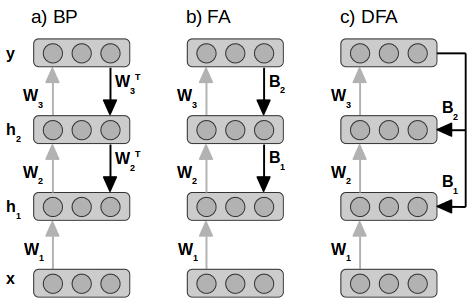
The basic idea of Feedback Alignment (FA) [1] is to use different matrices for the forward and backward pass of the backpropagation. Moreover, the matrices used for the backward pass are fixed and random. Let me elaborate. Recall how backpropagation works:
- Propagate the input from the input layer to the output layer via hidden layers (forward pass).
- Calculate the loss.
- Propagate the error backwards from the output layer to the hidden layers (backward pass).
The matrices used for propagation in step 1 and step 3 are the same - the weights of the model. In step 3, once you have the error at layeri, you multiply it with the layer's parameters to get the error for the layeri-1 (ignoring details like propagating error through the activation function). But one could say that steps 1 and 3 have two different matrices which happen to be identical and remain identical throughout the training. What FA does is introduce new random matrices for step 3 and keep them fixed throughout the training. So you calculate the loss at the output layer and randomly project it back to the hidden layers to train the network. And this works! It's surprising because the parameters of the network receive some random projection of the loss, and they somehow learn to make use of it. For this, they need to change in a way that the randomly projected loss makes sense for them and propels them towards values which solve the training task at hand. You probably also understand the name "Feedback Alignment" now. The parameters learn to "align" with the "feedback" received via fixed random matrices.
A follow-up work by Arild Nøkland proposed the "Direct Feedback Alignment" (DFA) [2] method where the error is directly propagated from the output layer to each individual hidden layer. To reach layer i, the error doesn't need to go through the layers i+1 to n which are closer to the output layer. This works as well and has an added advantage that the layers can be trained in parallel.
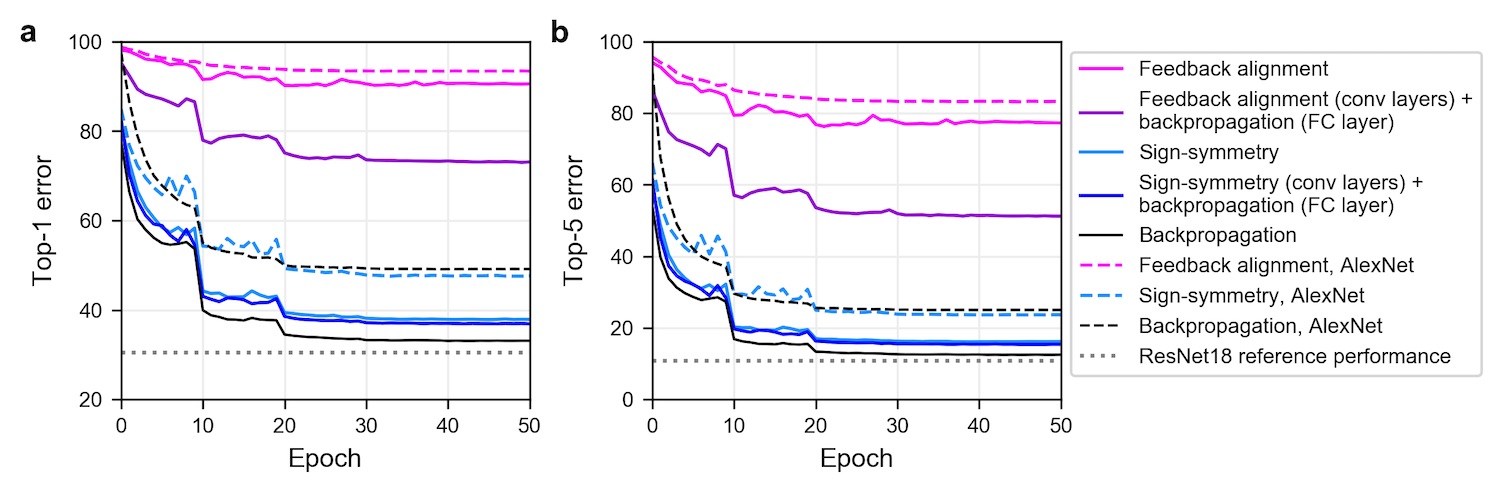
While FA does perform reasonably well on MNIST and CIFAR, it fails to do so on ImageNet with large networks. But one can make this work by relaxing the relation (or rather the lack of it) between weights used for the forward and backward pass. Xiao et al. [3] and Moskovitz et al. [4] show that if you use "sign-concordant feedback" from Liao et al. [5], FA can perform almost as good as backpropagation. What sign-concordance/sign-symmetry means is that the signs(+/-) of the weights used for the forward and backward pass should be the same, i.e. the magnitude of the parameters used for the backward pass are still fixed and random but share the sign with the parameters used for the forward pass. So it's really just the signs of the parameters that matter! Fig 2 below from Xiao et al. [3] shows how sign-concordant feedback performs nearly as well backpropagation. We'll see the importance of the signs of the parameters later as well.
Predicting the future while training a network
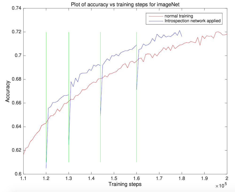
"Introspection: Accelerating neural network training by learning weight evolution" by Sinha et al. [6] shows something exciting: you can predict what the value of a parameter is going to be far in training while training the network before you reach that point! It's one obvious implication is that you can reduce the training time by directly jumping to the future values of the parameters. How much? Well, that, of course, depends on how good the predictor (of future parameter values) is, when (during the training) can you make the jump, and how far. You should check the paper for answers to these and other similar questions but, in short, there's no golden rule (yet) to make these choices, and they need to be determined empirically. But that is how any work in a particular direction starts. The first attempt requires quite some manual tuning, and the results are not that awesome, but things improve over time. Results get better, and it gets easier to finetune hyperparameters. That's how it happened, for instance, for object detection. But let's not meander and come back to the paper. The way the "future value predictor" works is that it looks at the trajectory of each parameter individually and predicts the future trajectory just like you'd do in time-series forecasting. To be more precise, it looks at a bunch of past values, not the whole trajectory and predicts one future value for a particular timestamp instead of forecasting the whole trajectory.
Two other things in the paper I found as amazing as the main idea are:
- The predictor (which they call introspection network) is really small in size. It's a fully-connected network with just one hidden layer with 40 neurons. The input layer has 4 neurons, and the output layer has 1.
- The predictor was trained ONLY on the trajectories of the parameters of a network trained on MNIST. The network trained on MNIST comprises of 3 convolutional layers and 2 fully-connected layers. The introspection network is still able to predict the trajectories of networks being trained on CIFAR and ImageNet.
The paper is easy to read. I'd encourage you to do that if you're interested in the details and the results they obtain. Some open questions which remain unanswered are:
- Would the introspection network perform better with its training data generated differently?
- Would the introspection network be better if it's trained on MNIST + CIFAR + ImageNet?
- Can the initial drop in the accuracy, when the jump is made, really be explained by how weights relate to each other?
- And most importantly, how far can you take this idea? Can it be used to reduce the training time significantly for training on gigantic datasets?
The only other work I'm aware of (which by the way this paper also cites) which goes in the direction of predicting "future" of training is Synthetic Gradients [7]. The basic idea there was to predict the gradients for a network's module (e.g. a layer) and train that module on them instead of training on the real gradients. The gradient predictors are then trained on the true gradients received later in the backward pass.
Exploration of the lottery ticket hypothesis
Zhou et al. in [8] analyse various aspects of the popular Lottery Ticket (LT) Hypothesis [9] and why it works. They present some intriguing results. I can't mention all of them in this section so I'll just talk about the most important ones. But before I do that, let's briefly recap LT so that we're on the same page. Before LT, the only thing we knew was that if you train a (big) network (typically with high weightage for L1 loss added to its loss function), you can prune it and get rid of a huge percentage of its parameters. You'd need to retrain/tune the pruned-network / sub-network a bit, but you won't lose any performance (accuracy). You will, as a result, get a small sub-network with a performance level similar to that of the bigger one. But if you try to train this small sub-network from scratch, its performance won't get anywhere close to that of the bigger network. Using LT algorithm, however, you can train the sub-network from scratch and still achieve similar performance. The trick is to initialise the sub-network with the exact same initial-values it had as part of the bigger original network. If you're training it on a big dataset like ImageNet, then you'd need to pick the values from epoch X (X=6 for ResNet-50 trained on ImageNet) as the initial values. Let's get back to the main paper now.
When I refer to a sub-network or a pruned network, I'd mean the network obtained by training a network and removing some of its weights based on some criterion. The paper presents analyses for many criteria like:
- Large weight values
- Large weight values whose sign didn't change during training
- A large increase in magnitude
- etc.
The things I found most striking in the paper are:
- It's the signs (+/-) of the initial weights of the sub-network that matter and not the magnitude. You can even assign all the weights a constant value (while taking care of the signs of course) and still achieve performance comparable to that of the original bigger network! So the magic is not in parameters' initial VALUES but initial SIGNS. In section 1, we talked about how signs of the weights matter for backpropagation; now we see that they also matter while training a pruned network from scratch. Signs of the weights seem magical!
- The other interesting thingy in the paper is what authors call "supermasks" ("mask" because one can define the architecture of a sub-network using a mask). They observed that the weights of the sub-network, when reverted to their initial values (not just signs), perform better than chance without any training! It doesn't end there. If you train the mask instead of training the network, you can obtain masks whose corresponding sub-networks perform almost as good as the original bigger network without any training. You should read section 5.1 of the paper if you're interested in how they train the mask instead of training the network.

The supermasks, and especially training the masks to get supermasks, remind me of Weight agnostic neural networks [10]. The basic idea in that work is to perform a Neural Architecture Search (NAS) while keeping the weights same. Usually, one would train a network (or a part of it) while performing NAS to check if the current architecture is good or not but in this work, researchers skip "training of the weights" part. The architectures found with this approach perform well without any training of the weights. The initial values, just like in the case of supermarks, are good enough. However, the process of NAS is, of course, more complicated than finding supermasks.
One major open question in [8] is whether all of this can generalise to other datasets like ImageNet, COCO etc. I hope this question gets answered in some follow-up work.
Deep Image Prior
Ulyanov et al. in [11] try to prove that certain generator network architectures possess an inductive bias for images. They show that just the architecture of these networks is sufficient to capture patterns in images. They do so by performing denoising, superresolution, and inpainting tasks without training a network on a dataset.
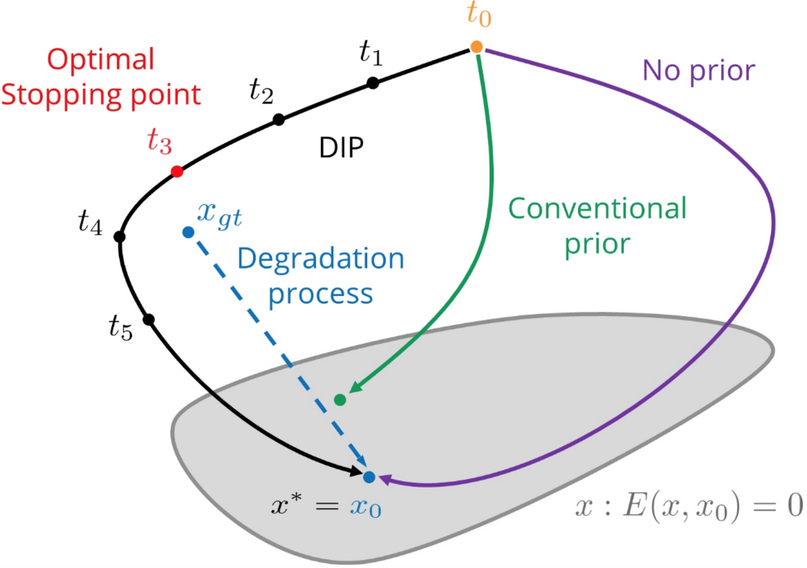
Their method is easy to understand. Let me explain it with the help of the denoising task. Denoising an image, as the name suggests, requires removing noise from a noisy image. What you do is provide a noisy image as an input to the network and "train" it to reproduce that noisy image. That's it! You "train" the network on that single image. I say "train" in quotes because training usually implies training the network on the whole dataset, not a single image. Here, backpropagation is performed on a randomly initialised network using only that one image you'd like to denoise. After some iterations, the network first produces (outputs) the image without noise, and as you perform more gradient steps, it eventually overfits and outputs the noisy input image. Fig 5 (from the IJCV version of the paper) below explains it using the trajectory of the parameters.
For superresolution, you'd ask it to produce a bigger image and then calculate the loss by downsampling the image. For the inpainting task, you'd ask the network to reproduce the image with some portion masked out. The authors note that the choice of architecture matters for the task at hand. If you read the paper, you'll get to see some fantastic results!
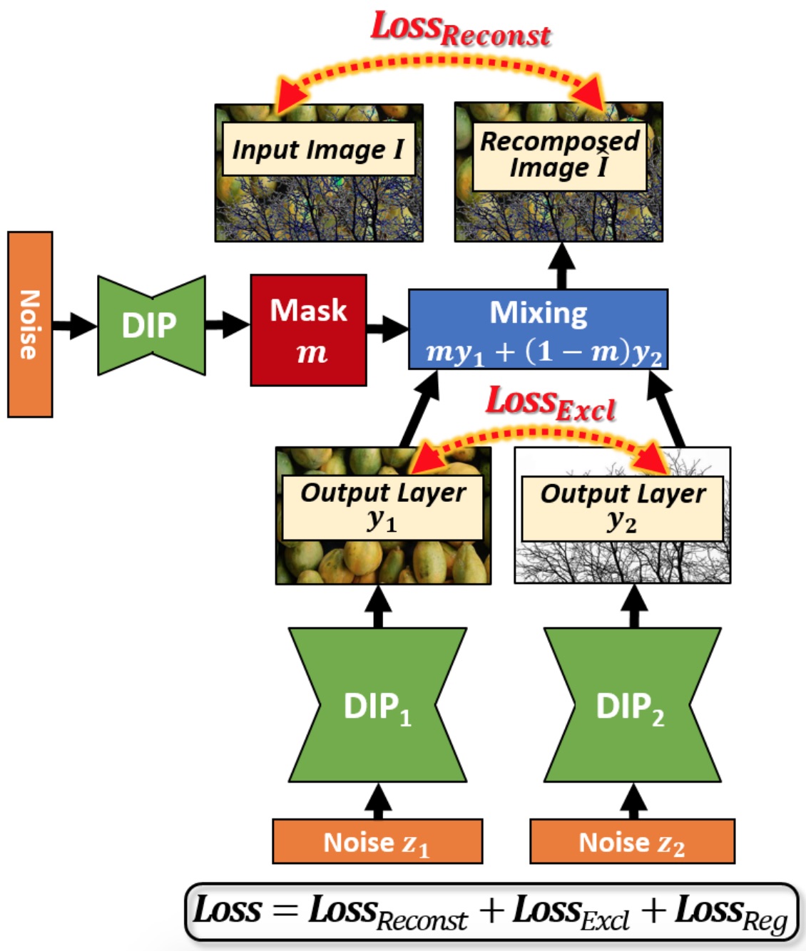
There was a follow-up work from Gandelsman et al. [12] which extends the capabilities of this method even further. They show that you can perform Image-Dehazing, Foreground/Background Segmentation, Watermark-Removal, and Transparency Separation if you use two DIP (Deep Image Prior) networks instead of one. Images in these tasks have two components (foreground/background, watermark/original-image, etc.) which can be separated using two DIP networks. The basic idea is that if you train two DIP networks to reproduce the input image together by combining their outputs, the image produced by each DIP network would contain one of the two components of the image. The way you combine the two outputs is by producing a pixel-wise mask using a third DIP network and masking out some pixels from 1st output and other pixels from the 2nd output. Their results are also staggering!
Key Takeaways
- The signs (+/-) of the parameters hold vital importance. They might be more critical than the magnitudes of the parameters.
- The parameters of a network follow a predictable trajectory. This predictive nature of the parameters allows us to jump ahead in training.
- Some architectures possess a strong inductive bias for images meaning that these architectures have some knowledge built into them.
References
- Lillicrap TP, Cownden D, Tweed DB, Akerman CJ. Random feedback weights support learning in deep neural networks. arXiv preprint arXiv:1411.0247. 2014 Nov 2.
- Nøkland A. Direct feedback alignment provides learning in deep neural networks. Advances in neural information processing systems. 2016;29:1037-45.
- Xiao W, Chen H, Liao Q, Poggio T. Biologically-plausible learning algorithms can scale to large datasets. arXiv preprint arXiv:1811.03567. 2018 Nov 8.
- Moskovitz TH, Litwin-Kumar A, Abbott LF. Feedback alignment in deep convolutional networks. arXiv preprint arXiv:1812.06488. 2018 Dec 12.
- Liao Q, Leibo JZ, Poggio T. How important is weight symmetry in backpropagation?. arXiv preprint arXiv:1510.05067. 2015 Oct 17.
- Sinha A, Sarkar M, Mukherjee A, Krishnamurthy B. Introspection: Accelerating neural network training by learning weight evolution. arXiv preprint arXiv:1704.04959. 2017 Apr 17.
- Jaderberg M, Czarnecki WM, Osindero S, Vinyals O, Graves A, Silver D, Kavukcuoglu K. Decoupled neural interfaces using synthetic gradients. InInternational Conference on Machine Learning 2017 Jul 17 (pp. 1627-1635). PMLR.
- Zhou H, Lan J, Liu R, Yosinski J. Deconstructing lottery tickets: Zeros, signs, and the supermask. InAdvances in Neural Information Processing Systems 2019 (pp. 3597-3607).
- Frankle J, Carbin M. The lottery ticket hypothesis: Finding sparse, trainable neural networks. arXiv preprint arXiv:1803.03635. 2018 Mar 9.
- Gaier A, Ha D. Weight agnostic neural networks. InAdvances in Neural Information Processing Systems 2019 (pp. 5364-5378).
- Ulyanov D, Vedaldi A, Lempitsky V. Deep image prior. InProceedings of the IEEE Conference on Computer Vision and Pattern Recognition 2018 (pp. 9446-9454).
- Gandelsman Y, Shocher A, Irani M. double-dip”: Unsupervised image decomposition via coupled deep-image-priors. InThe IEEE Conference on Computer Vision and Pattern Recognition (CVPR) 2019 Jun (Vol. 6, p. 2).